Training and making prediction for a single allele

Load packages

Note that if you have installed the epinb package, then you do not need (and probably won’t want) to run sys.path.append("..").

import sys
sys.path.append("..")

import epinb

import pandas as pd

Read in training data

The training data we used are from Keskin et al. You can substitute it with any data, be they your house data or other public data.

training_data = pd.read_csv("../data/keskin/Keskin peptide lists filtered.csv")
training_data

	Allele	Length	Peptide
0	A0101	8	ADMGHLKY
1	A0101	8	ELDDTLKY
2	A0101	8	FSDNIEFY
3	A0101	8	FTELAILY
4	A0101	8	GLDEPLLK
...	...	...	...
186459	G0104	24	SASSLGGGFGGGSRGFGGASGGGY
186460	G0104	26	GSGGSSYGSGGGSYGSGGGGGGHGSY
186461	G0104	27	LLLPLLLLLLLLLGAGVPGAWGQAGSL
186462	G0104	27	QEESLRQEYAATTSRRSSGSSCNSTRR
186463	G0104	28	QEGETIELDKPVMAEGNVEVWLNSLLEE

186464 rows × 3 columns

Train the model

As an example, we train a model for A0203.

model = epinb.NBScore() # Create a model.
model = model.fit(training_data.loc[training_data['Allele'] == 'A0203', 'Peptide'])

Read in the test data

The test data are curated from IEDB. The positive examples are the experimentally verified binders. The negative examples are randomly generated from the source proteins. The ratio of positive to negative data is 1:99.

test_data = pd.read_csv("../data/test-data/IEDB-A0203.txt", header=None, names=["peptide", 'label'])
test_data

	peptide	label
0	FGGHIRSV	pos
1	YLNSVVQV	pos
2	ILHDVVEV	pos
3	ALGSVVAV	pos
4	FLATIMGV	pos
...	...	...
259595	LVPDYGMSNLT	neg
259596	LLGEATEGRIS	neg
259597	NCKCLKTLSVS	neg
259598	LLTRGDMRECV	neg
259599	RLLEKVEGTVR	neg

259600 rows × 2 columns

Make the prediction

We use predict_log_odds to make the predicion.

res = model.predict_log_odds(test_data['peptide'])
res

array([ 10.50781303,  40.28167703,  41.24288408, ..., -35.1040942 ,
        -5.85900102, -35.84848082])

Interpretation

1st-order motifs

First, we can inspect the trained model by looking at the scoring matrices. First of all, we can check the 1st order motifs by using fit_details_1.

model.fit_details_1().round(3)

	1	2	3	4	5	7	8	9	0
A	0.139	0.009	0.164	0.052	0.051	0.011	0.098	0.076	0.093
C	0.002	0.000	0.000	0.002	0.005	0.001	0.007	0.007	0.003
D	0.000	0.000	0.002	0.157	0.038	0.003	0.012	0.013	0.000
E	0.002	0.000	0.003	0.187	0.060	0.009	0.062	0.111	0.001
F	0.111	0.001	0.131	0.012	0.065	0.023	0.010	0.024	0.003
G	0.075	0.002	0.017	0.089	0.086	0.017	0.023	0.075	0.001
H	0.021	0.000	0.025	0.016	0.077	0.004	0.031	0.022	0.001
I	0.055	0.070	0.107	0.013	0.078	0.217	0.048	0.011	0.113
K	0.051	0.001	0.139	0.040	0.086	0.010	0.058	0.074	0.000
L	0.068	0.737	0.020	0.022	0.084	0.298	0.126	0.046	0.246
M	0.016	0.079	0.025	0.003	0.010	0.022	0.025	0.012	0.004
N	0.026	0.000	0.047	0.049	0.045	0.010	0.044	0.046	0.000
P	0.000	0.000	0.026	0.146	0.022	0.105	0.043	0.009	0.000
Q	0.021	0.030	0.019	0.042	0.040	0.012	0.065	0.095	0.001
R	0.046	0.000	0.056	0.016	0.061	0.007	0.071	0.057	0.000
S	0.147	0.002	0.063	0.080	0.048	0.014	0.085	0.116	0.004
T	0.063	0.012	0.024	0.040	0.033	0.029	0.092	0.125	0.006
V	0.067	0.056	0.038	0.020	0.067	0.200	0.087	0.043	0.523
W	0.004	0.000	0.003	0.005	0.014	0.001	0.003	0.003	0.000
Y	0.086	0.000	0.092	0.010	0.030	0.009	0.010	0.034	0.000

To see the log odds for an AA at a given location, use what='log_odds'.

model.fit_details_1(what='log_odds').round(3)

	1	2	3	4	5	7	8	9	0
A	0.579	-2.159	0.749	-0.400	-0.415	-1.963	0.227	-0.020	0.178
C	-1.891	-6.002	-3.604	-2.289	-1.206	-2.958	-0.750	-0.750	-1.491
D	-4.821	-4.821	-3.505	1.083	-0.320	-2.824	-1.512	-1.417	-7.219
E	-3.500	-5.034	-3.169	1.045	-0.092	-2.034	-0.060	0.527	-4.387
F	1.006	-3.516	1.170	-1.178	0.465	-0.585	-1.385	-0.502	-2.687
G	0.077	-3.552	-1.395	0.253	0.217	-1.418	-1.085	0.087	-4.050
H	-0.077	-6.371	0.108	-0.328	1.221	-1.756	0.315	-0.041	-3.326
I	-0.069	0.174	0.596	-1.526	0.279	1.299	-0.204	-1.654	0.652
K	-0.148	-4.290	0.846	-0.396	0.367	-1.809	-0.027	0.221	-4.937
L	-0.339	2.037	-1.557	-1.483	-0.139	1.132	0.274	-0.739	0.942
M	-0.424	1.203	0.060	-2.024	-0.893	-0.071	0.060	-0.711	-1.803
N	-0.494	-7.003	0.088	0.129	0.063	-1.438	0.028	0.071	-7.003
P	-4.699	-7.096	-0.603	1.133	-0.767	0.801	-0.092	-1.612	-7.096
Q	-0.608	-0.285	-0.723	0.066	0.028	-1.148	0.502	0.881	-3.875
R	-0.137	-7.211	0.055	-1.193	0.155	-2.013	0.296	0.083	-7.211
S	0.747	-3.377	-0.104	0.147	-0.373	-1.628	0.199	0.515	-2.873
T	0.129	-1.516	-0.841	-0.308	-0.498	-0.648	0.515	0.822	-2.174
V	0.008	-0.176	-0.560	-1.212	0.002	1.098	0.262	-0.445	2.058
W	-1.101	-5.717	-1.322	-0.841	0.172	-2.283	-1.206	-1.454	-5.717
Y	1.016	-6.686	1.085	-1.160	-0.038	-1.243	-1.121	0.084	-4.288

2nd order motifs

Similarly, you can check the frequencies, log odds, and the difference between the frequency and the expected values without correlation \(P(ab) - P(a)P(b)\).

model.fit_details_2().round(3)

	20	12	57	23	10	90	35	80	30	24	37	34	58	89	45	38	78	49	79	15
AA	0.0	0.002	0.001	0.001	0.016	0.009	0.011	0.011	0.015	0.001	0.004	0.011	0.007	0.006	0.003	0.016	0.001	0.005	0.001	0.007
AC	0.0	0.000	0.000	0.000	0.000	0.001	0.001	0.000	0.002	0.000	0.000	0.000	0.000	0.000	0.000	0.000	0.000	0.000	0.000	0.000
AD	0.0	0.000	0.000	0.000	0.000	0.000	0.003	0.000	0.000	0.001	0.000	0.019	0.000	0.001	0.002	0.003	0.000	0.001	0.000	0.004
AE	0.0	0.000	0.000	0.000	0.000	0.000	0.005	0.000	0.000	0.001	0.001	0.033	0.004	0.009	0.003	0.006	0.000	0.004	0.001	0.008
AF	0.0	0.000	0.000	0.003	0.000	0.000	0.013	0.001	0.000	0.000	0.003	0.003	0.001	0.005	0.004	0.002	0.000	0.001	0.000	0.009
...	...	...	...	...	...	...	...	...	...	...	...	...	...	...	...	...	...	...	...	...
YS	0.0	0.000	0.000	0.000	0.000	0.000	0.005	0.000	0.001	0.000	0.000	0.006	0.003	0.001	0.001	0.006	0.001	0.000	0.001	0.005
YT	0.0	0.002	0.000	0.000	0.002	0.000	0.002	0.000	0.000	0.000	0.003	0.003	0.002	0.001	0.000	0.006	0.000	0.001	0.002	0.001
YV	0.0	0.005	0.004	0.000	0.037	0.015	0.003	0.007	0.042	0.000	0.016	0.002	0.001	0.001	0.001	0.007	0.002	0.000	0.000	0.009
YW	0.0	0.000	0.000	0.000	0.000	0.000	0.002	0.000	0.000	0.000	0.000	0.001	0.000	0.000	0.000	0.000	0.000	0.000	0.000	0.000
YY	0.0	0.000	0.000	0.000	0.000	0.000	0.005	0.000	0.000	0.000	0.001	0.001	0.000	0.001	0.000	0.001	0.000	0.000	0.000	0.003

400 rows × 20 columns

model.fit_details_2('log_odds').round(3)

	20	12	57	23	10	90	35	80	30	24	37	34	58	89	45	38	78	49	79	15
AA	-2.663	-1.347	-1.627	-1.627	0.958	0.337	0.612	0.577	0.908	-1.627	-0.446	0.577	0.081	0.020	-0.798	0.982	-2.017	-0.265	-1.627	0.137
AC	-3.462	-3.462	-3.462	-3.462	-3.462	-0.417	-0.028	-1.064	0.252	-3.462	-3.462	-3.462	-1.064	-3.462	-3.462	-1.064	-3.462	-1.064	-3.462	-1.064
AD	-4.678	-2.281	-4.678	-4.678	-4.678	-4.678	-0.284	-4.678	-4.678	-1.244	-4.678	1.538	-2.281	-1.634	-0.568	-0.416	-4.678	-1.244	-4.678	0.031
AE	-4.892	-4.892	-4.892	-4.892	-4.892	-4.892	0.057	-2.494	-4.892	-1.847	-1.458	1.866	-0.182	0.551	-0.629	0.126	-2.494	-0.182	-1.458	0.412
AF	-4.409	-4.409	-4.409	-0.015	-2.012	-4.409	1.422	-0.975	-4.409	-4.409	0.101	-0.015	-0.975	0.386	0.300	-0.478	-4.409	-0.975	-4.409	1.033
...	...	...	...	...	...	...	...	...	...	...	...	...	...	...	...	...	...	...	...	...
YS	-4.032	-4.032	-1.635	-4.032	-1.635	-4.032	0.843	-4.032	-0.598	-4.032	-4.032	0.985	0.230	-0.988	-0.988	0.985	-0.598	-1.635	-0.988	0.763
YT	-3.800	-0.086	-3.800	-3.800	-0.086	-3.800	0.132	-3.800	-1.402	-3.800	0.595	0.463	0.132	-0.366	-3.800	1.217	-1.402	-0.755	-0.086	-0.366
YV	-3.993	0.882	0.622	-3.993	2.854	1.976	0.402	1.149	3.002	-3.993	2.026	-0.061	-0.559	-0.559	-0.948	1.260	-0.279	-3.993	-3.993	1.450
YW	-2.261	-2.261	-2.261	-2.261	-2.261	-2.261	1.850	-2.261	-2.261	-2.261	-2.261	0.784	-2.261	-2.261	0.137	-2.261	-2.261	0.137	-2.261	0.137
YY	-3.230	-3.230	-3.230	-3.230	-0.832	-3.230	1.566	-3.230	-3.230	-3.230	-0.185	0.204	-3.230	-0.185	-3.230	0.204	-3.230	-0.832	-3.230	1.165

400 rows × 20 columns

model.fit_details_2('surplus').round(4)

	20	12	57	23	10	90	35	80	30	24	37	34	58	89	45	38	78	49	79	15
AA	-0.0004	0.0003	0.0006	-0.0003	0.0030	0.0015	0.0028	0.0018	-0.0001	0.0007	0.0021	0.0023	0.0016	-0.0012	0.0000	0.0003	-0.0003	0.0007	0.0003	-0.0001
AC	-0.0000	0.0000	-0.0000	-0.0000	-0.0005	0.0005	0.0004	0.0000	0.0010	-0.0000	-0.0001	-0.0003	0.0000	-0.0007	-0.0002	-0.0008	-0.0001	0.0000	-0.0001	-0.0003
AD	0.0000	0.0003	-0.0002	-0.0000	0.0000	0.0000	-0.0032	0.0000	0.0000	-0.0002	-0.0005	-0.0063	-0.0002	-0.0005	0.0003	0.0008	-0.0001	0.0005	-0.0001	-0.0011
AE	-0.0000	-0.0001	-0.0004	-0.0000	-0.0001	-0.0001	-0.0044	0.0003	-0.0001	-0.0009	-0.0002	0.0028	0.0011	-0.0019	-0.0004	-0.0043	-0.0003	-0.0015	-0.0000	-0.0005
AF	-0.0000	-0.0002	-0.0012	0.0019	0.0000	-0.0002	0.0026	0.0009	-0.0004	-0.0001	-0.0002	0.0011	0.0006	0.0023	0.0009	0.0003	-0.0001	-0.0001	-0.0003	-0.0000
...	...	...	...	...	...	...	...	...	...	...	...	...	...	...	...	...	...	...	...	...
YS	0.0000	-0.0002	-0.0000	0.0000	0.0001	-0.0001	0.0006	-0.0000	0.0008	0.0000	-0.0013	-0.0016	0.0002	-0.0004	0.0003	-0.0020	0.0004	-0.0007	-0.0003	0.0006
YT	0.0000	0.0005	-0.0009	0.0000	0.0010	-0.0002	-0.0011	-0.0001	-0.0002	0.0000	0.0005	-0.0010	-0.0008	-0.0001	-0.0003	-0.0027	-0.0004	-0.0004	0.0004	-0.0017
YV	0.0000	0.0002	-0.0021	0.0000	-0.0084	-0.0025	-0.0030	0.0013	-0.0058	0.0000	-0.0025	0.0001	-0.0014	0.0007	0.0001	-0.0006	0.0008	-0.0004	-0.0004	0.0032
YW	0.0000	0.0000	-0.0000	0.0000	0.0000	0.0000	0.0010	0.0000	0.0000	0.0000	-0.0001	0.0003	-0.0001	-0.0000	0.0003	-0.0003	-0.0000	0.0004	-0.0000	-0.0008
YY	0.0000	0.0000	-0.0003	0.0000	0.0004	-0.0000	0.0019	-0.0000	-0.0000	0.0000	-0.0000	0.0003	-0.0003	0.0004	-0.0003	0.0002	-0.0001	0.0001	-0.0003	0.0005

400 rows × 20 columns

You can also order the table by the values and look at the top ones by using the argument topk. It will return two tables, one for the amino acid combinations, and one for the values.

motifs = model.fit_details_2('log_odds', topk=5)
display(*motifs)

	20	12	57	23	10	90	35	80	30	24	37	34	58	89	45	38	78	49	79	15
0	LV	FL	HI	LF	FV	QV	FH	QV	FV	LP	FP	YP	HQ	HQ	PH	YH	IQ	EQ	LQ	FH
1	MV	YL	HL	LY	YV	TV	FG	HV	YV	LE	YP	FP	HT	HT	DH	FK	IT	PQ	IT	YH
2	LL	SL	HV	LK	SV	SV	YH	VV	AV	LD	KI	FD	HL	RQ	EH	FH	IH	PT	VQ	SH
3	LI	AL	HP	LA	AV	EV	AH	RV	KV	MP	YL	KD	FH	QQ	PW	FT	IS	DQ	IQ	AH
4	IV	TL	NI	LI	GV	KV	SH	TV	IV	LN	FL	KE	WV	SQ	EK	YQ	LQ	DE	IS	FW

	20	12	57	23	10	90	35	80	30	24	37	34	58	89	45	38	78	49	79	15
0	3.968404	2.995305	2.618943	3.133074	2.959139	2.944130	2.528115	2.531336	3.121548	3.144728	2.876409	2.806752	2.049579	1.560612	2.506171	1.700219	1.862923	2.101606	2.167193	2.305801
1	3.323167	2.989770	2.405264	2.996197	2.854202	2.881966	2.122911	2.455499	3.002108	3.123856	2.448491	2.460102	1.818278	1.532253	2.154133	1.628834	1.851526	2.094137	2.081669	2.102378
2	3.115853	2.785283	2.182888	2.846397	2.733449	2.759961	2.102378	2.445432	2.727398	3.026109	2.408002	2.209447	1.697751	1.408893	2.078523	1.616795	1.841238	2.005926	1.969686	2.084538
3	2.733461	2.594956	1.755693	2.817257	2.576541	2.476866	2.001333	2.439247	2.679017	2.366761	2.353638	2.140911	1.696202	1.383627	1.943675	1.609359	1.819307	1.971862	1.960324	1.940892
4	2.528408	2.180415	1.727443	2.440064	2.324494	2.306427	1.955743	2.413481	2.672438	2.244819	2.225964	2.085642	1.487226	1.371914	1.838149	1.553519	1.720833	1.855554	1.946959	1.586144

You can easily consolidate the two tables.

motifs[0] + ' ' + motifs[1].round(2).astype(str)

	20	12	57	23	10	90	35	80	30	24	37	34	58	89	45	38	78	49	79	15
0	LV 3.97	FL 3.0	HI 2.62	LF 3.13	FV 2.96	QV 2.94	FH 2.53	QV 2.53	FV 3.12	LP 3.14	FP 2.88	YP 2.81	HQ 2.05	HQ 1.56	PH 2.51	YH 1.7	IQ 1.86	EQ 2.1	LQ 2.17	FH 2.31
1	MV 3.32	YL 2.99	HL 2.41	LY 3.0	YV 2.85	TV 2.88	FG 2.12	HV 2.46	YV 3.0	LE 3.12	YP 2.45	FP 2.46	HT 1.82	HT 1.53	DH 2.15	FK 1.63	IT 1.85	PQ 2.09	IT 2.08	YH 2.1
2	LL 3.12	SL 2.79	HV 2.18	LK 2.85	SV 2.73	SV 2.76	YH 2.1	VV 2.45	AV 2.73	LD 3.03	KI 2.41	FD 2.21	HL 1.7	RQ 1.41	EH 2.08	FH 1.62	IH 1.84	PT 2.01	VQ 1.97	SH 2.08
3	LI 2.73	AL 2.59	HP 1.76	LA 2.82	AV 2.58	EV 2.48	AH 2.0	RV 2.44	KV 2.68	MP 2.37	YL 2.35	KD 2.14	FH 1.7	QQ 1.38	PW 1.94	FT 1.61	IS 1.82	DQ 1.97	IQ 1.96	AH 1.94
4	IV 2.53	TL 2.18	NI 1.73	LI 2.44	GV 2.32	KV 2.31	SH 1.96	TV 2.41	IV 2.67	LN 2.24	FL 2.23	KE 2.09	WV 1.49	SQ 1.37	EK 1.84	YQ 1.55	LQ 1.72	DE 1.86	IS 1.95	FW 1.59

If you want all combinations sorted, simply use topk=400.

motifs = model.fit_details_2('log_odds', topk=400)
motifs[0] + ' ' + motifs[1].round(2).astype(str)

	20	12	57	23	10	90	35	80	30	24	37	34	58	89	45	38	78	49	79	15
0	LV 3.97	FL 3.0	HI 2.62	LF 3.13	FV 2.96	QV 2.94	FH 2.53	QV 2.53	FV 3.12	LP 3.14	FP 2.88	YP 2.81	HQ 2.05	HQ 1.56	PH 2.51	YH 1.7	IQ 1.86	EQ 2.1	LQ 2.17	FH 2.31
1	MV 3.32	YL 2.99	HL 2.41	LY 3.0	YV 2.85	TV 2.88	FG 2.12	HV 2.46	YV 3.0	LE 3.12	YP 2.45	FP 2.46	HT 1.82	HT 1.53	DH 2.15	FK 1.63	IT 1.85	PQ 2.09	IT 2.08	YH 2.1
2	LL 3.12	SL 2.79	HV 2.18	LK 2.85	SV 2.73	SV 2.76	YH 2.1	VV 2.45	AV 2.73	LD 3.03	KI 2.41	FD 2.21	HL 1.7	RQ 1.41	EH 2.08	FH 1.62	IH 1.84	PT 2.01	VQ 1.97	SH 2.08
3	LI 2.73	AL 2.59	HP 1.76	LA 2.82	AV 2.58	EV 2.48	AH 2.0	RV 2.44	KV 2.68	MP 2.37	YL 2.35	KD 2.14	FH 1.7	QQ 1.38	PW 1.94	FT 1.61	IS 1.82	DQ 1.97	IQ 1.96	AH 1.94
4	IV 2.53	TL 2.18	NI 1.73	LI 2.44	GV 2.32	KV 2.31	SH 1.96	TV 2.41	IV 2.67	LN 2.24	FL 2.23	KE 2.09	WV 1.49	SQ 1.37	EK 1.84	YQ 1.55	LQ 1.72	DE 1.86	IS 1.95	FW 1.59
...	...	...	...	...	...	...	...	...	...	...	...	...	...	...	...	...	...	...	...	...
395	AS -4.95	EA -4.89	SG -4.83	KL -5.01	EA -4.89	LD -4.89	EG -4.77	SG -4.83	LT -4.93	TL -4.93	EA -4.89	EA -4.89	PD -4.17	II -4.51	YL -4.36	EG -4.77	AD -4.68	VI -4.63	GK -4.68	EV -4.74
396	KL -5.01	AE -4.89	AE -4.89	EL -5.1	LT -4.93	AE -4.89	ES -4.78	LR -4.88	LK -5.01	GA -4.94	VA -4.91	LI -5.0	EF -4.24	AP -4.56	VP -4.4	GE -4.77	DA -4.68	LP -4.77	AD -4.68	PL -4.77
397	LK -5.01	AG -4.94	EA -4.89	GL -5.16	AG -4.94	AG -4.94	GS -4.83	LD -4.89	LE -5.1	EL -5.1	LK -5.01	LK -5.01	PE -4.39	GV -4.79	FA -4.41	GG -4.83	EG -4.77	AI -4.79	GV -4.79	ES -4.78
398	EL -5.1	AS -4.95	AS -4.95	SL -5.16	LE -5.1	LG -5.16	DL -4.89	AG -4.94	LG -5.16	GL -5.16	LE -5.1	EL -5.1	VD -4.53	GG -4.83	RE -4.5	LD -4.89	GG -4.83	IA -4.79	EA -4.89	EA -4.89
399	GL -5.16	LE -5.1	SA -4.95	AL -5.27	EL -5.1	LS -5.16	EA -4.89	LE -5.1	LS -5.16	SL -5.16	LA -5.27	LV -5.12	GD -4.56	DL -4.89	LE -5.1	EL -5.1	AG -4.94	LD -4.89	AL -5.27	EL -5.1

400 rows × 20 columns

Evaluation

To evaluate the results, we need some utilities from scikit-learn. To install, in your terminal, activate the virtual environment you are running for this note book, and run conda install scikit-learn.

from sklearn.metrics import roc_curve, roc_auc_score, auc, precision_recall_curve
import matplotlib.pyplot as plt
import bisect

test_data['prediction'] = res
test_data

	peptide	label	prediction
0	FGGHIRSV	pos	10.507813
1	YLNSVVQV	pos	40.281677
2	ILHDVVEV	pos	41.242884
3	ALGSVVAV	pos	25.334613
4	FLATIMGV	pos	39.310739
...	...	...	...
259595	LVPDYGMSNLT	neg	-34.499987
259596	LLGEATEGRIS	neg	-31.344300
259597	NCKCLKTLSVS	neg	-35.104094
259598	LLTRGDMRECV	neg	-5.859001
259599	RLLEKVEGTVR	neg	-35.848481

259600 rows × 3 columns

fpr, tpr, roc_thresholds = roc_curve(test_data.label, test_data['prediction'],
                                     pos_label='pos')
auroc = auc(fpr, tpr)

precision, recall, pr_thresholds = precision_recall_curve(test_data.label, test_data['prediction'],
                                     pos_label='pos')

ind_40_tpr = bisect.bisect(tpr, 0.4) # fpr = recall
def fpr_tpr_to_precision(fpr, tpr, neg_pos_ratio):
    return tpr / (neg_pos_ratio * fpr + tpr)
prec_at_40_tpr = fpr_tpr_to_precision(fpr[ind_40_tpr], tpr[ind_40_tpr], 99)

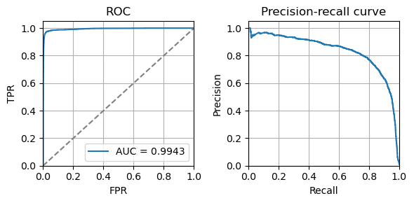
print(f"AUROC: {auroc:.4f}; Precision at 40% recall: {prec_at_40_tpr:.4f}")

AUROC: 0.9943; Precision at 40% recall: 0.9146

plt.figure(figsize=(6, 3))
plt.subplot(1, 2, 1)

plt.plot(fpr, tpr, label = "AUC = %0.4f" % auroc)
plt.plot([0, 1], [0, 1], color="grey", linestyle="--")
plt.grid('both')
plt.xlim([0.0, 1.0])
plt.ylim([0.0, 1.05])
plt.xlabel('FPR')
plt.ylabel('TPR')
plt.title("ROC")
plt.legend(loc="lower right")

plt.subplot(1, 2, 2)
plt.plot(recall, precision, label = "AUC = %0.4f" % auroc)
plt.grid('both')
plt.xlim([0.0, 1.0])
plt.ylim([0.0, 1.05])
plt.xlabel('Recall')
plt.ylabel('Precision')
plt.title("Precision-recall curve")

plt.tight_layout()

Visualization

For visualization, we need two additional packages: logomaker for motif logo and wordcloud for word clouds.

Logo plots

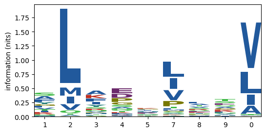
We use logo plots for 1st order motifs

import logomaker
from scipy.stats import entropy

temp = model.fit_details_1().T.reset_index(drop=True)
temp = temp * (3 - entropy(temp.T).reshape([-1, 1]))

fig, ax = plt.subplots(1, 1, figsize=[6, 3])
ww_logo = logomaker.Logo(temp,
                         color_scheme='NajafabadiEtAl2017',
                        ax=ax,
                         vpad=.1,
                         width=.8)
ww_logo.ax.set_xticks([0, 1, 2, 3, 4, 5, 6, 7, 8], [1, 2, 3, 4, 5, 7, 8, 9, 0])
ww_logo.ax.set_ylabel('information (nits)')
# ww_logo.ax.set_ylim([0, 3])
display(ww_logo)

<logomaker.src.Logo.Logo at 0x7f9223ee9d00>

Word clouds

We use word clouds for 2nd order motifs

import wordcloud

wc = wordcloud.WordCloud(width = 800, height = 375, min_font_size = 10, background_color ='white', collocations=False)
wc.fit_words(model.fit_details_2()['20'].to_dict())
plt.imshow(wc)
plt.axis("off")

(-0.5, 799.5, 374.5, -0.5)